Probit modeling via MCMCpack

I thought briefly about doing a survey of Bayesian R packages in my book. I'm sure a comparative survey would be helpful to many users, but it is difficult to cover all of the packages in any depth in a 30 page chapter. Also, since packages are evolving so fast, much of what I could say would quickly be out of date.

One package that looks attractive is the MCMCpack package written by Andrew Martin and Kevin Quinn. They provide MCMC algorithms for many popular statistical models and it seems, at first glance, easy to use.

Since I just demonstrated the use of Gibbs sampling for a probit model with a normal prior, let's fit this model by MCMCpack.

The appropriate R function to use is MCMCprobit which uses the same Albert-Chib sampling algorithm-- in it's most basic form, the function looks like

fit = MCMCprobit(model, data, burnin, mcmc, thin, b0, B0)

Here

fit: is a description of the probit model, written as any R model like lm.
data: is the data frame that is used
burnin: is the number of iterations for the burnin period
mcmc: is the number of Gibbs iterations
thin: is the thinning interval
b0: is the prior mean of the multivariate prior
B0: is the prior precision matrix

For my model, here is the syntax:

fit=MCMCprobit(success~prev.success+act, data=as.data.frame(DATA), burnin=0,
mcmc=10000, thin=1, b0=prior$beta, B0=prior$P)

After it is run, one can get summaries of the simulated draws of beta by the summary command.

summary(fit)

Iterations = 1:10000
Thinning interval = 1
Number of chains = 1
Sample size per chain = 10000

1. Empirical mean and standard deviation for each variable,
plus standard error of the mean:

Mean SD Naive SE Time-series SE
(Intercept) -1.53215 0.75595 0.0075595 0.0110739
prev.success 1.03590 0.24887 0.0024887 0.0038060
act 0.05093 0.03700 0.0003700 0.0005172

2. Quantiles for each variable:

2.5% 25% 50% 75% 97.5%
(Intercept) -3.03647 -2.03970 -1.53613 -1.02398 -0.04206
prev.success 0.54531 0.86842 1.03246 1.20129 1.52685
act -0.02117 0.02567 0.05132 0.07559 0.12451

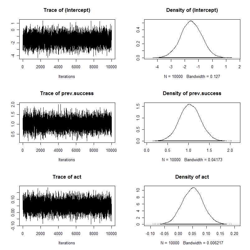
Also, one can get trace plots and density estimates by the plot command.

plot(command)

What do I think about this particular function in MCMCpack?

1. The execution time for the MCMC is much faster using MCMCprobit since the sampling is done using compiled C++ code. How much faster? For 10,000 iterations of Gibbs sampling, it took my laptop 0.58 seconds to do this sampling in MCMCpack compared with 4.53 seconds using my R function.

2. MCMCprobit allows for more user input such as the burnin period, thinning rate, starting values, random number seed, etc.

3. It allows one to output latent residuals (Albert and Chib, Biometrika) and compute marginal likelihoods by the Laplace method.

Generally, the function worked fine and I got essentially the same results as I had before. My only quibble is that it took two tries for MCMCprobit to run. It complained that my prior precision matrix was not symmetric, although I computed this matrix by the var command in R. There was a quick fix -- I rounded the values of this matrix to two decimal places and MCMCprobit didn't complain.